numpy pandas2
Numpy and pandas are two basic tools for data analysis using python. Numpy is used more in linear algebra, while pandas is more used to analyze table-structured data. Both numpy and pandas have one-dimensional and two-dimensional data structures.
Numpy one-dimensional arrays are called arrays. The definition is as follows:
import numpy as np
a=np.array([1,2,3,4,5])
There are also a few basic applications:
#查询元素
a[0]
#切片访问
a[1:3]
#循环访问
for i in a:
   print(i)
#数据类型
a.dtype
We can find that List and array one-dimensional arrays look very similar, so what is the difference between them?
numpy is suitable for data analysis because it has many features that List does not have:
(1) Statistical function
#求平均值
a.mean()
#求标准差
a.std()
#向量相加
a=np.array([1,2,3])
b=np.array([4,5,6])
a+b
a*b
The one-dimensional data structure of pandas is called series. The definition is as follows:
import pandas as pd
stocks=pd.Series([54.74,190.9,173.14,1050.3,181.86,1139.49],
index=['Tencent','Alibaba','Apple','Google','Facebook','Amazon'])
If the array one-dimensional array is similar to the List, then the Series is similar to the Dictionary, and each index value corresponds to a value. Series is an upgraded version of array one-dimensional array, with many functions that it does not have:
#获取描述统计信息
stocks.describe()
#运用iloc属性根据位置获取值
stocks.iloc[1]
#运用loc属性根据索引值获取值
stocks.loc['腾讯']
#根据索引值进行向量的加减乘除,若索引值不对应,则会产生数值型缺失值NaN
s1=pd.Series([1,2,3,4],index=['a','b','c','d'])
s2=pd.Series([10,20,30,40],index=['a','b','e','f'])
s3=s1+s2
s3
#那出现缺失值了,如何删除呢
s3.dropna()
s3
Let's take a look at the two-bit data structure, which has both rows and columns.
Numy uses array to create two-dimensional arrays, while Pandas uses DataFrame to create two-dimensional arrays.
Let's first look at a few simple operations of array two-dimensional array:
#定义二维数组(创建一个三行四列二维数组)
a=np.array([
           [1,2,3,4],
           [5,6,7,8],
           9,10,11,12]
                      ])
#查询元素 前面代表行号,后面代表列号
a[0,2]
#获取第一行
a[0,:]
#获取第一列
a[:,0]
#计算平均值、标准差的办法(array一维数组则没有这个功能)
 #计算整个数组所有元素的平均值/标准差
a.mean()
a.std()
  #计算每一行的平均值/标准差
a.mean(axis=1)
a.std(axis=1)
  #计算每一列的平均值/标准差
a.mean(axis=0)
a.std(axis=0)
Let's take a look at the Pandas two-dimensional array DataFrame, which is very similar to our Excel.
The following is its simple operation:
#第一步需要定义字典
salesDict={'购药时间':['2008-01-01 星期五','2018-01-01 星期六','2018-01-06 星期三'],
          '社保卡号':['001616528','001616528','001616528'],
          '商品编码':[236701,236701,236701],
          '商品名称':['强力VC银翘片','清热解毒口服液','感康'],
          '销售数量':[6,1,2],
          '应收金额':[82.8,28,16.8],
          '实收金额':[69,24.64,15]}
salesDf=pd.DataFrame(salesDict)
salesDf
#但由于字典是无序的,如果需要让它按照我们输入的键排列的话,就需要定义有序字典
from collections import OrderedDict
salesOrderedDict=OrderedDict(salesDict)
salesDf=pd.DataFrame(salesOrderDict)
#平均值计算,按每列来求
salesDf.mean()
#运用iloc属性根据位置获取值,前面代表行号,后面代表列号
salesDf.iloc[0,1]
  #获取第一行
salesDf.iloc[0,:]
  #获取第一列
salesDf.iloc[:,0]
#运用loc属性根据索引值获取值,前面代表行名,后面代表列名
salesDf.loc[0,'商品编码']
    #获取第一行
salesDf.loc[0,:]
    #获取第一列
salesDf.iloc[:,'商品名称']
#查询范围
  #查询某几列
salesDf.[['商品名称'],['销售数量']]
  #查询指定连续的列
salesDf.loc[:,'商品名称','销售数量']
#通过条件判断筛选符合条件的行
querySer=salesDf.loc[:,'销售数量']>1
querySer
salesDf.loc[querySer,:]
#查看数据有多少行和列
salesDf.shape
#查看每一列的统计数
salesDf.describe()
Below we introduce the basic process of data analysis:
There are 5 steps in total, which are asking questions / understanding data / data cleaning / building models / data visualization
First ask the question: We intend to ask for the dataset: Chaoyang Hospital's 2018 sales data
Monthly average consumption times/monthly average consumption amount/customer unit price
understanding the data
#读取数据
FileNameStr='./朝阳医院2018年销售数据'
xls=pd.ExcelFile(FileNameStr,dtype='object') salesDf=xls.parse('Sheet1',dtype='object')
Then perform data cleaning:
There are 6 small steps in this step, which are selecting subset/column name renaming/missing data processing/data type conversion/data sorting/outlier processing
#选择子集
subsalesDf=salesDf.loc[0:4,'购药时间':'销售数量']
subsalesDf
#列名重命名 前面是旧列名,后面是新列名,inplace=True是将原数据框变成新数据框,
  而False则是创建一个改动的新数据框
colNameDict={'购药时间':'销售时间'}
salesDf.rename(columns=colNameDict,inplace=True)
#缺失数据处理 选取的列数值有缺失就会被删掉
salesDf=salesDf.dropna(subset=['销售时间','社保卡号'],how='any')
#数据类型转换
salesDf['销售数量']=salesDf['销售数量'].astype('float')
salesDf['应收金额']=salesDf['应收金额'].astype('float')
salesDf['实收金额']=salesDf['实收金额'].astype('float')
print('转换后的数据类型:\n',salesDf.dtypes)
#分割销售日期 ,将'2008-01-01 星期五'分割,取'2008-01-01'
def splitSaletime(timeColSer):
    timeList=[]
    for value in timeColSer:
          dateStr=value.split('')[0]
          timeList.append(dateStr)
    timeSer=pd.Series(timeList)
     return timeSer
timeSer=salesDf.loc[:,'销售时间']
dateSer=splitSaletime(timeSer)
#修改销售时间这一列的值
salesDf.loc[:,'销售时间']=dateSer
#字符串转换日期
salesDf.loc[:,'销售时间']=pd.to_datetime(salesDf.loc[:,'销售时间'],
                                        format='%Y-%m-%d',
                                         errors='coerce')
#将转换日期过程中不符合日期格式的数值转换而成的空值None删除掉
salesDf=salesDf.dropna(subset=['销售时间','社保卡号'],how='any')
#将数据排序 ascending=True表示升系,False降序
salesDf=salesDf.sort_values(by='销售时间',ascending=True)
#排列后行数顺序会乱,所以要重命名
salesDf=salesDf.reset_index(drop=True)
#异常值处理 通过条件判断筛选出我们想要的数据
querySer=salesDf.loc[:,'销售数量']>0
salesDf=salesDf.loc[querySer,:]
Then build the model:
Average monthly consumption = total consumption/month
(The consumption of the same social security card number on the same day is counted as this consumption)
#删除重复数据
kpi1Df=salesDf.drop_duplicates(subset=['销售时间','社保卡号'])
#查看kpi1Df总共有多少行,即总消费次数
totalkpi1Df=kpi1Df.shape[0]
#按销售时间排序并重命名
kpi1Df=kpi1Df.sort_value(by='销售时间',ascending=True)
kpi1Df=kpi1Df.reset_index(drop=True)
#获取时间范围
startTime=kpi1Df.loc[0,'销售时间']
endTime=kpi1Df.loc[totalkpi1Df-1,'销售时间']
#计算月份数
days=(endTime-startTime).days
months=days//30
#总消费次数/月份数
kpi1=totalkpi1Df//months
Average monthly consumption amount = total consumption amount / total number of months
#总消费金额
totalMoney=salesDf.loc[:,'实收金额'].sum()
#总消费金额/总月份数
monthMoney=totalMoney/months
Customer unit price = total consumption amount / total consumption times
pct=totalMoney/kpi1The final step is data visualization to reflect changing trends. This requires the use of the matplotlib drawing tool. Let's listen to the next decomposition.
When I was learning this content, after I defined the split function splitSaletime, I called the function to display an error, as shown in the following figure:
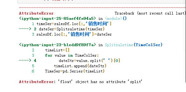
With the help of the great god, I learned that the reason is because the data in my column contains data with missing values of floating-point data type, so I used the dropna function to delete it... and succeeded.
The content of this piece of data analysis is relatively basic and easy to understand. It also allows me to master a skill for data analysis outside of excel, and compared to excel, it is more comfortable to use python after memorizing the code ~ life is too short, I use python !